An AI conveyor belt in NVIDIA Isaac Sim - Part 2 (Synthetic Data Generation)
Introduction
Welcome to Part 2 - generating synthetic data to train the ML model.
The goal of this step is to generate images for the classifier, which will identify objects on the conveyor belt.
The code in this part was adapted from the Isaac Sim standalone example for online learning data generation, but I’ve simplified it for this experiment. There are some things like bounding boxes in the ground truth I’m not interested in.
(If you just want to see the code you can find it here).
What this post will describe:
- How to set up an environment to place objects and render images for the training dataset.
- How to load ShapeNet models into the environment.
- How to use the Isaac Sim Data Randomization (DR) features to randomize the domain.
The goal of a synthetic dataset is to re-create the circumstances in which objects will be observed in “real life”. For synthetic data generation, this means a rendering environment which is very close to reality or photo-realistic. For this experiment I’m not going to do anything in actual reality, but do want to explore some of these concepts.
In an ideal world, if we wanted to identify an object on a conveyor belt, the camera would be perfectly placed, there would be only one light source with a known location, and the object would be perfectly aligned:
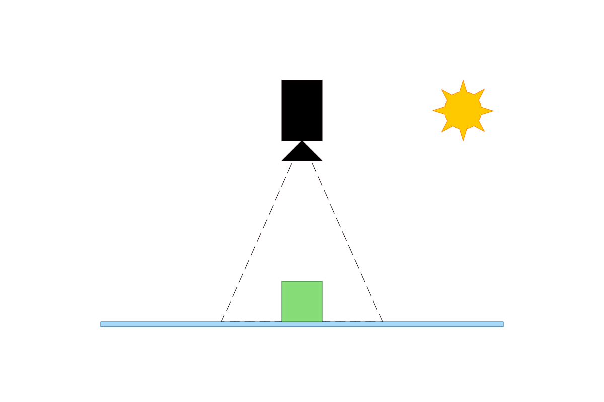
But in real life this isn’t practical:
- The light source would be variable (e.g. sunlight changes through the day).
- There could be multiple light sources.
- The object won’t be aligned to the camera direction.
- The object will not be in the middle of the camera.
- etc.
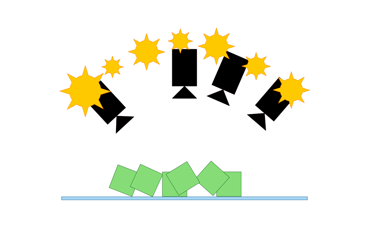
Domain Randomization (DR) is used to vary the synthetic data generation to make the object detection algorithm more robust. In this example I’ll be:
- Varying the light location.
- Varying the light intensity.
- Varying the camera orientation.
- Varying the object orientation.
- Varying the object position.
We can also use data augmentation to supplement the training data, e.g. translating, scaling & rotating captured 2D images, but it is better to use DR in the 3D environment. Why? Transforming 2D training images cannot change the lighting of the 3D model, and shadows are useful information - data augmentation cannot create the correct shadows. But let’s leave that for Part 3.
With DR we will generate these kind of images:
There is more we could do:
- Add more lights.
- Vary the the object material.
- Vary the belt material.
- etc.
Isaac Sim has comprehensive support for randomizing the simulation is a wide variety of ways, I’m only exploring a few of these here.
Set up the environment
For both the camera and light, we add an extra Xform object so it’s easier to rotate around the origin, instead of rotating the light or camera itself.
The conveyor belt is flat plate with similar color to what we’ll be using (see Part 1).
There are 3 DR commands:
- One that varies the light position (rotates around origin), using the “rig”.
- One that varies the light intensity.
- One that varies the camera position using the “rig”.
1
2
3
4
5
6
7
8
9
10
11
12
13
14
15
16
17
18
19
20
21
22
23
24
25
26
27
28
29
30
31
32
33
34
35
36
37
38
39
40
41
42
43
44
45
46
47
48
49
50
51
52
53
54
55
56
57
58
59
from omni.isaac.core.utils.prims import create_prim
from omni.isaac.core.utils.rotations import euler_angles_to_quat
import omni.isaac.dr as dr

# Camera and rig
create_prim(
    "/World/CameraRig",
    "Xform"
)
create_prim(
    "/World/CameraRig/Camera",
    "Camera",
    position=np.array([0.0, 0.0, 100.0])
)

# Light source
create_prim("/World/LightRig", "Xform")
create_prim(
    "/World/LightRig/Light",
    "SphereLight",
    position=np.array([100, 0, 200]),
    attributes={
        "radius": 50,
        "intensity": 5e4,
        "color": (1.0, 1.0, 1.0)
    }
)

# Conveyor "belt"
create_prim(
    "/World/Belt",
    "Cube",
    position=np.array([0.0, 0.0, -1.0]),
    scale=np.array([100.0, 100.0, 1.0]),
    orientation=euler_angles_to_quat(
        np.array([0.0, 0.0, 0.0]),
        degrees=True
    ),
    attributes={"primvars:displayColor": [(0.28, 0.65, 1.0)]},
)

# DR commands for light and camera
dr.commands.CreateLightComponentCommand(
    light_paths=["/World/LightRig/Light"],
    intensity_range=(5e3, 5e4),
    seed=dr_seed()
).do()
dr.commands.CreateRotationComponentCommand(
    prim_paths=["/World/LightRig"],
    min_range=(0.0, 15.0, -180.0),
    max_range=(0.0, 60.0, 180.0),
    seed=dr_seed()
).do()
dr.commands.CreateRotationComponentCommand(
    prim_paths=["/World/CameraRig"],
    min_range=(0.0, 0.0, -180.0),
    max_range=(0.0, 60.0, 180.0),
    seed=dr_seed()
).do()
Load a ShapeNet object
There are some details you can find in the code regarding ShapeNet files, and please refer to the NVIDIA example if you want to run this code. NB: There is a script to convert the ShapeNet files the USD files which must be run first for the appropriate categories.
1
2
3
4
5
6
7
8
9
10
11
12
13
14
15
16
17
18
19
20
21
22
23
24
25
26
27
28
29
30
31
32
33
34
35
36
37
38
39
40
41
42
43
44
45
46
47
48
49
50
51
52
from pxr import UsdGeom
import omni.isaac.dr as dr
from omni.isaac.core.utils.prims import create_prim
from omni.isaac.core.utils.rotations import euler_angles_to_quat
from omni.isaac.core.prims.xform_prim import XFormPrim
from omni.isaac.core.materials import PreviewSurface

asset_reference = random.choice(self.asset_references[category])

# Create the shape
create_prim("/World/Shape", "Xform")
prim = create_prim(
    "/World/Shape/Mesh",
    "Xform",
    scale=np.array([20.0, 20.0, 20.0]),
    orientation=euler_angles_to_quat(
        np.array([90.0, 0.0, 0.0]),
        degrees=True),
    usd_path=asset_reference,
    semantic_label=category)

# Determine bounds and translate to sit on the Z=0 plane
primX = XFormPrim("/World/Shape/Mesh")
orientation_on_plane = euler_angles_to_quat(
    np.array([90.0, 0.0, 0.0]),
    degrees=True)
primX.set_local_pose(
    np.array([0.0, 0.0, 0.0]),
    orientation_on_plane)
bounds = UsdGeom.Mesh(prim).ComputeWorldBound(0.0, "default")
new_position = np.array([0.0, 0.0, -bounds.GetBox().GetMin()[2]])
primX.set_local_pose(new_position)

# Create a material and apply it to the shape
material = PreviewSurface(
    prim_path="/World/Looks/ShapeMaterial",
    color=np.array([0.2, 0.7, 0.2]))
primX.apply_visual_material(material)

# Add the translate and rotate DR commands
dr.commands.CreateMovementComponentCommand(
    prim_paths=["/World/Shape"],
    min_range=(-5.0, -5.0, 0.0),
    max_range=(5.0, 5.0, 0.0),
    seed=dr_seed()
).do()
dr.commands.CreateRotationComponentCommand(
    prim_paths=["/World/Shape"],
    min_range=(0.0, 0.0, 0.0),
    max_range=(0.0, 0.0, 360.0),
    seed=dr_seed()
).do()
Capturing the RGB ground truth
Capturing the ground truth is as simple as setting the default viewport to the camera and using the SyntheticDataHelper. The helper can capture other ground truths like image segmentation and and bounding boxes, which is useful if you have multiple objects in the same image.
I’m not sure why multiple generator.world.step() calls is required - I have discovered this helps with rendering artifacts but I’m still looking for a solution that isn’t a workaround.
1
2
3
4
5
6
7
8
9
10
11
12
13
14
15
16
17
18
19
20
21
22
import omni.isaac.dr as dr
from omni.kit.viewport import get_default_viewport_window
from omni.isaac.synthetic_utils import SyntheticDataHelper

viewport = get_default_viewport_window()
viewport.set_active_camera("/World/CameraRig/Camera")
viewport.set_texture_resolution(1024, 1024)
sd_helper = SyntheticDataHelper()

sd_helper.initialize(sensor_names=["rgb"], viewport=viewport)

dr.commands.RandomizeOnceCommand().do()
generator.world.step()
generator.world.step()
generator.world.step()

ground_truth = sd_helper.get_groundtruth(
    ["rgb"],
    viewport, verify_sensor_init=True
)
image = Image.fromarray(ground_truth["rgb"])
image.save(filename)
The randomization can happen either by running the simulation or manually calling the randomize command. NB the Data Randomization must be set to manual mode by toggling it exactly once:
1
dr.commands.ToggleManualModeCommand().do()
The results
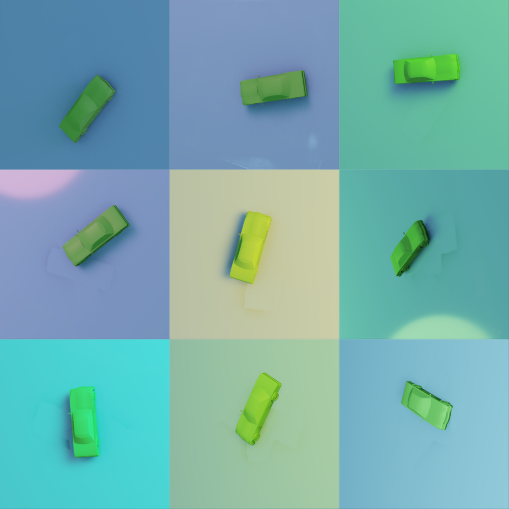
Here’s what 9 images look like for one shape category. You can see the variation in position, rotation, lighting and camera angle. Note there are still some rendering artifacts from the previous car position which needs to be fixed:
You can look at the full code for generating multiple datapoints here.
Next steps
Using these images I will train a Tensorflow classifier. I’m not TOO concerned with accuracy, 90%+ should be fine for the goals of this experiment. And then once I have the classifier I will integrate it into the simulation so we can sort objects from the conveyor belt.